Everything You Need to Know About Table Pivot in Excel

Making sense of large data sets is a challenge that many professionals face daily. Whether managing financial reports or tracking sales performance, understanding trends and patterns is important. The need for quick, efficient, and clear data insights has never risen before like now. Imagine being able to transform raw data into organized and actionable summaries within minutes.

This is where table pivot in Excel comes in, designed for dynamic data management shine. It allows you to sort and summarize information dynamically and save valuable time while offering unmatched flexibility in data analysis. Thus, this article will guide you through everything you need to know to understand the fundamentals to unlock this advanced feature.

Part 1. What is an Excel Pivot Table?

An Excel pivot table is a feature designed to transform raw data into meaningful insights. Users can filter and reorganize their data interactively, helping them easily uncover patterns and trends. Alongside that, this tool eliminates the hassle of manually calculating totals or percentages by automating these tasks.

Furthermore, it enables you to focus on decision-making instead of struggling with complex calculations. You can customize data views to suit your specific needs and make it a powerful ally for professionals and students alike. Whether dealing with sales metrics or project management tasks, this feature makes analysis faster and more intuitive.

Part 2. Different Use Cases of Table Pivot in Excel

Now that you understand what Pivot Table is and how it works, let's explore its practical applications across various scenarios. This powerful tool can be applied in various industries and tasks to enhance your ability to analyze data quickly. Below, we will explore some use cases where pivot tables can be helpful.

• Sales Analysis: You can track sales performance across regions, products, and time periods. It helps you identify trends or measure growth and make strategic decisions based on accurate data insights.
• Financial Reporting: This feature lets you summarize income or expenses and enables you to prepare accurate profit-and-loss statements. Users can also customize views that help them identify spending patterns and optimize budgeting.
• Customer Data Management: By grouping customer data, you can analyze purchase patterns and behavior. A pivot table in Excel can help identify your best customers, frequency of purchase, and other valuable insights to improve marketing strategies.
• Employee Performance: Business owners can analyze their employees' data using performance metrics and productivity levels. Additionally, it helps you evaluate team performance and allocate resources more effectively.

Part 3. How to Create and Manage an Excel Pivot Table?

After exploring the various uses of pivot tables, you have to learn how to create and manage one. Understanding the process helps you unlock the full potential of your data and make analysis seamless. Thus, let's dive into the steps for creating and customizing an Excel pivot table:

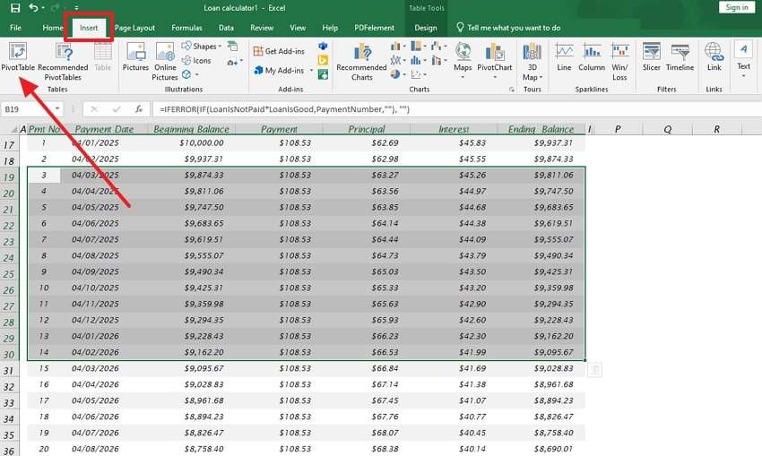
Step 1. To start the process, navigate the worksheet and select the data from which you want to create a pivot table. Then, you need to click on the “Insert” tab and choose the “Pivot Table” option from the newly appeared tools.

Step 2. After that, you will access the new dialog box where you have to type the “Table/Range” name. Next, choose the location where you want to save the newly generated pivot table and press the “OK” button to finish the process.

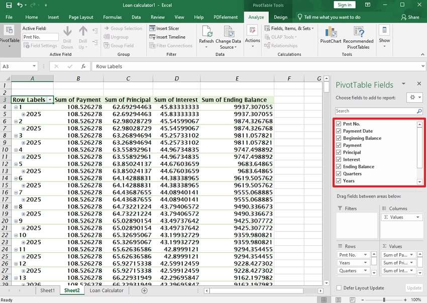
Step 3. Upon seeing the new interface, choose the “Fields” by checking it from the right-side panel of the screen. Now, your pivot table has been created and placed in its default fields.

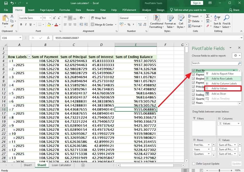
Step 4. If you want to change the default field area, right-click the “Field” and choose the “Add To Values” option or areas tailored to your preference.

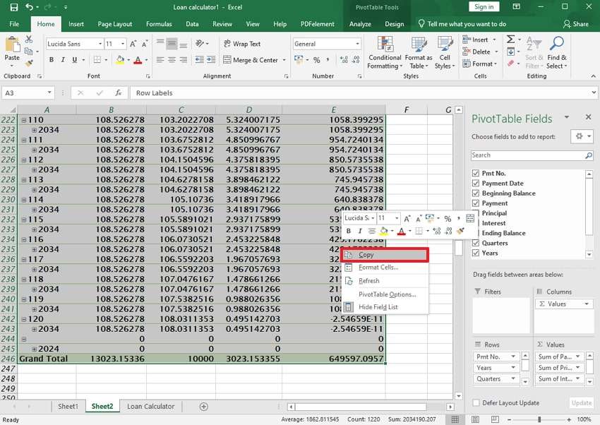
Step 5. Moving forward, select all the pivot tables or any area you want to copy and use. After that, right-click the table to access the Excel quick menu. Upon seeing it, choose the “Copy” option to copy all the selected text and paste it anywhere. Additionally, you can copy the content of the pivot table in Excel by pressing the “CTRL” and “C” buttons simultaneously.

Step 6. To sort a pivot table, simply choose the value and right-click on it. Upon accessing the pop-up, pick the “Sort” option and select “Sort Smallest to Largest” or vice versa, according to your preference.

Part 4. How to Create Excel Pivot Table Columns Area?

Upon creating a pivot table, understanding its components is important for effective data organization. The column area is vital in structuring your insights and allows you to group or compare data efficiently. In this section, we'll guide you through configuring the columns area to make the most of your Excel pivot table.

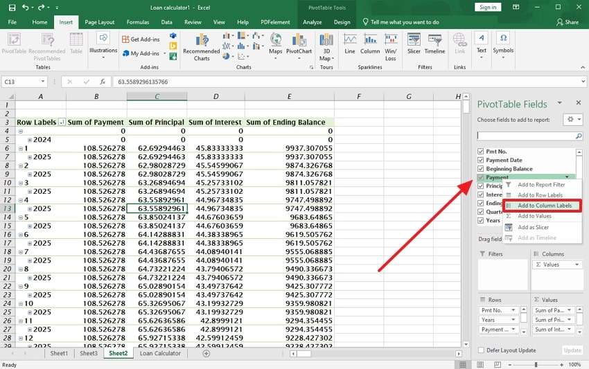
Instructions. To add a column area, you need to right-click the “Field” from the pivot table fields panel. Afterward, choose the “Add To Column Labels” option to create an Excel pivot table column area.

Part 5. How to Create an Excel Pivot Table with Multiple Columns?

After mastering the basics of the columns area, incorporating multiple columns adds depth to your analysis. This feature allows you to compare various data points and reveal comprehensive insights. Thus, follow the steps below to create a more detailed pivot table in Excel by adding multiple columns:

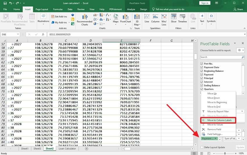
Step 1. Initiate this process by choosing the “Field” from the other area and clicking on it. Then, press the “Move to Column Labels” option to save the field list in the column area.

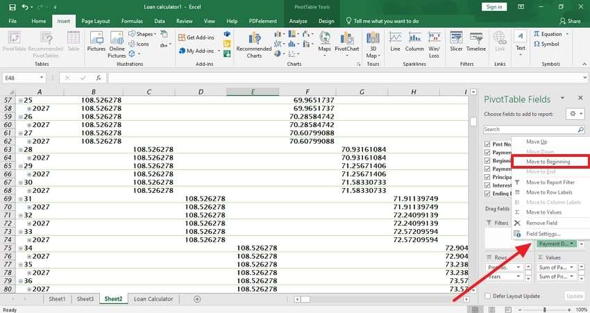
Step 2. Upon adding multiple fields in the column area, you can change the fields placed in the area. To do this, simply click the “Field” and choose “Move to Beginning” or other places as needed.

Part 6. How to Create a Calculated Field in an Excel Pivot Table?

Taking your pivot table skills further, calculated fields allow you to perform custom calculations directly within the table. This feature helps you derive new insights without modifying the original data source. Go through the guidelines below to learn how to create and use a calculated field to enhance your Excel pivot table:

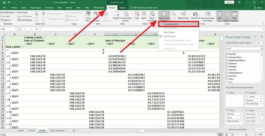
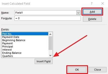
Step 1. Initiate the process by navigating to the “Analyze” tab and clicking the “Fields, Items & Sets” menu. Afterward, choose the “Calculated Fields” option from the newly appeared drop-down menu.

Step 2. Following this, you will access a dialog box where you need to input the “Name” and “Formula” of your field. Then, you can add pivot table field names by clicking the “Insert Field” button. Upon adding it, press the “OK” button to successfully create a calculated field in the pivot table.

Part 7. How to Manage Corrupted or Damaged Excel Files Without Losing Data?

When working with pivot tables in Excel, protecting your work from unexpected issues like file corruption is important. Despite taking all necessary precautions, files can become damaged due to factors such as system crashes or virus infections. When your spreadsheet or pivot table gets corrupted, it may become unreadable and put your valuable data at risk.

To repair the corrupt pivot table of Excel, we recommend Repairit for fixing corrupted or damaged files. This tool helps you repair broken Excel files without losing important data and makes it ideal where your pivot table is compromised. Furthermore, it works by scanning the damaged file, identifying issues, and restoring your valuable data.

Key Features of Repairit File Repair

1. Batch Repair: Users can repair multiple corrupted files simultaneously and boost productivity by handling several documents.
2. Virus Recovery: This tool lets you repair files damaged by viruses to ensure no data loss and files remain intact, including complex file structures.
3. Preview Files: It previews the restored content after repairing the file to confirm that all important data is accurately recovered.
4. ZIP Repair: You can fix corrupted or incomplete ZIP archives to extract files, verify hierarchy, and restore files even if they exceed 1GB.

Wondershare Repairit - Excel Repair

Try It Free Try It Free

1,010,994 people have downloaded it.

• Repair damaged Excel files with all levels of corruption, including blank files, files not opening, unrecognizable format, unreadable content, files layout changed, etc.

• Repairs all kinds of data stored in damaged Excel files such as tables, charts, formulas, comments, images, etc.

• Support all formats of Excel files: XLSX/XLSM/XLTX/XLTM/XLS

• Perfectly repair corrupted files with a very high success rate, without modifying the original file.

• No limit to the number and size of the repairable files.

• Support Windows 11/10/8/7/Vista, Windows Server 2003/2008/2012/2016/2019/2022, and macOS 10.12~macOS 13.

• Repairit also supports all formats of PDF, Word, Excel, PowerPoint, ZIP, and Adobe files.

Easiest Manual to Use Repairit to Manage Corrupted or Damaged Excel Files

Follow the comprehensive instructions below to understand how to use this file repair toolbox to repair a corrupt pivot table of Excel:

Step 1. Access this File Repair Toolbox to Initiate the Process

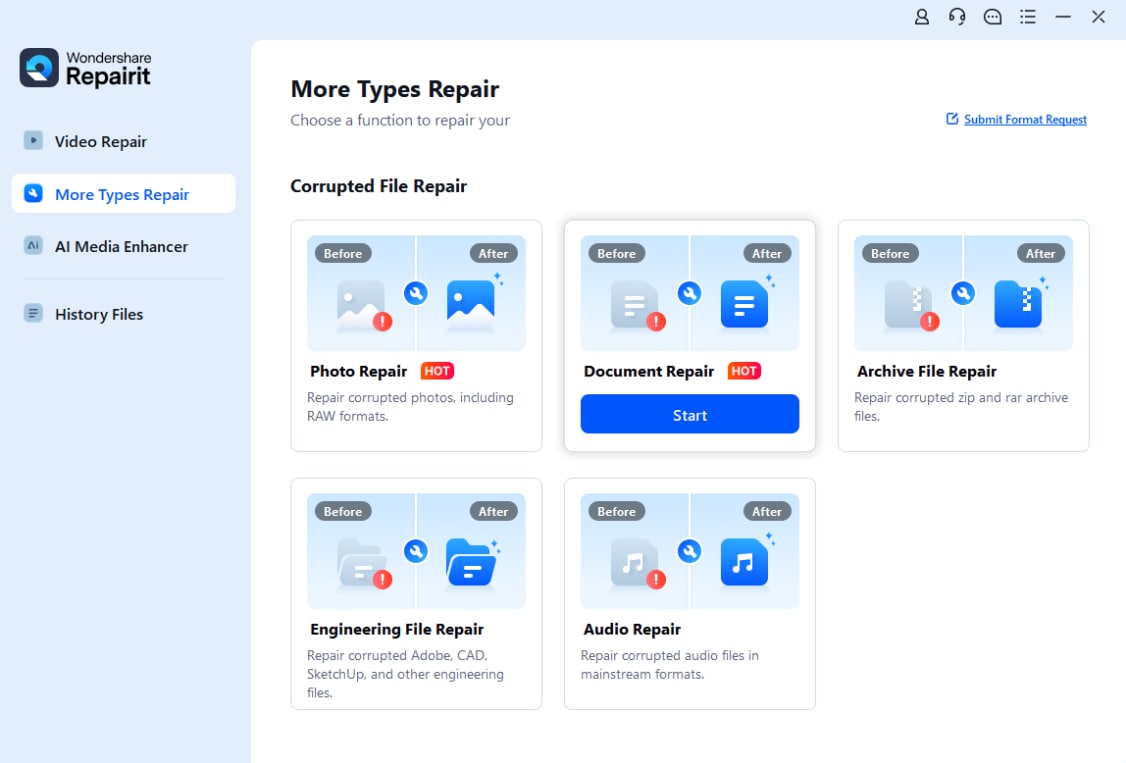
Upon downloading this advanced file repair tool, you need to launch it to commence the process. Next, locate and select the “More Types Repair” tab from the main interface on the screen. Within this menu, choose the “File Repair” feature to move further with the repair process.

Step 2. Import the Corrupted Excel File with Pivot Table

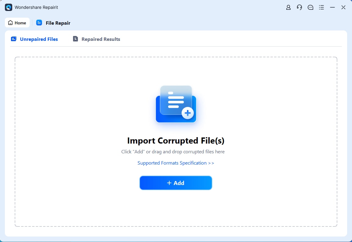
Afterward, press the “+ Add” button from the newly appeared interface.

Step 3. Initiate the Excel Repairing Procedure

Now, click the “Repair” button to begin the repair operation, and you will see a progress bar that may appear during the process.

Part 8. Tips and Tricks for Creating and Managing Pivot Tables in Excel

After covering how to create and manage pivot tables, you should know some more tips and tricks to make your experience more efficient. These strategies will help you enhance your data analysis and management skills. Furthermore, it lets you get the most out of your table pivot in Excel. Thus, let’s dive in to explore some important points to manage pivot tables more efficiently.

• Group Data for Better Insights: You can group data in pivot tables by categories such as months, years, or ranges. This feature allows you to analyze trends or perform time-based comparisons without altering the raw data.
• Use Calculated Fields for Custom Metrics: This is particularly useful for performing custom calculations directly on the pivot table and creating new data points, such as profit margins or growth rates. It saves time by eliminating the need to manually calculate these metrics outside the table.
• Refresh Pivot Table Data: To ensure you are always working with the most current information, you need to refresh the pivot table. For this, right-click the table pivot in Excel and select "Refresh" to pull in the latest data to ensure accurate analysis each time.
• Sort and Filter Data: You must use the sorting options to arrange data in ascending or descending order. This flexibility allows you to work with large datasets without feeling overwhelmed.

Conclusion

In short, pivot tables are a powerful tool for simplifying complicated data and stats. They provide a user-friendly way to transform raw information into actionable insights. Automating calculations and enabling flexible data customization saves time and effort for professionals and students alike. However, you may observe that while managing pivot tables in Excel, your file becomes corrupted or damaged.

To cater to these needs, we recommend you use Repairit, which ensures data security and recovery without hassle. Its capabilities, such as batch repair and preview options, ensure your data is restored without any loss. So, try Repairit today to safeguard your data and enjoy uninterrupted data analysis.