How To Correct N/A and #VALUE! Issues With Vlookup? [Plus Tips]

VLOOKUP, despite its usefulness, can often trip up even experienced data users. And if you are here, chances are, you also handle data in your profession. Most Excel users rely on VLOOKUP for quick information retrieval. It’s a handy tool, but issues with VLOOKUP often disrupt your workflow. Several reasons are behind it, including data mismatch, formatting, and formula errors.

So, whether you’re working in finance, marketing, or any other industry, we understand your challenges. This article will discuss the common VLOOKUP issues in Excel you might encounter. So, read on to learn how to fix them and best practices to enhance your spreadsheet skills.

Part 1: 12 Common Issues With VLOOKUP and Solutions To Tackle Them

When working with numbers and formulas in spreadsheets, you might face problems, like issues with VLOOKUP. The common errors are #N/A and #VALUE. Let’s explore what causes these errors and find solutions to handle them confidently.

Issue 1: #N/A Errors Due to Text vs. Number Formatting

VLOOKUP expects consistency, so any mismatch leads to the #N/A error. This VLOOKUP issue in Excel usually happens when your lookup values aren’t formatted the same. If the lookup column has inconsistent formatting, such as one set as text and the other as numbers, VLOOKUP might not find a match.

Solution: Convert the Format From Text to Number

Before using VLOOKUP, ensure your lookup values and the corresponding column in the table have the same data type. Here’s how to change from Text to Number format:

Step 1: Select the column you need to change in the Excel spreadsheet.

Step 2: Right-click and choose Format Cells to open the settings in a pop-up window.

Step 3: Go to the Number tab, select Number under the Category section, and choose a format without leading zeros.

Step 4: Click OK to apply the changes.

Issue 2: Leading/Trailing Spaces Causing Incorrect Matches

One of the most common VLOOKUP format issues is when extra spaces are present in your data. These spaces can cause mismatches, leading to inaccurate results or #N/A errors. Imagine you have a table of product names and their corresponding prices:

You want to use VLOOKUP to find the price of “Apple (Extra Sweet).” However, there is a trailing space in the product name cell.

When you use the formula =VLOOKUP("Apple (Extra Sweet)", A1:B4, 2, FALSE), Excel returns "#N/A". It is because the trailing space makes the product name different from the one in the table, even though they appear visually identical.

Solution 1: Using the TRIM function

Remove the spaces from your lookup values and the table array. Use the TRIM function in Excel to eliminate any leading or trailing spaces.

Example:

=VLOOKUP(TRIM("Apple (Extra Sweet)"), TRIM(A1:A4), 2, FALSE)

You can also use the CLEAN function instead of TRIM, which removes extra characters like non-printing characters.

Solution 2: Removing Spaces Manually

Here’s how to remove leading/trailing spaces:

Step 1: Select the product name cells containing spaces.

Step 2: Go to the Home tab and click Find & Select in the upper navigation pane.

Step 3: The Find and Replace pop-up window will open. Go to the Replace tab and enter a space in the Find what text field.

Step 4: Leave the Replace with text field blank.

Step 5: Click Replace All to remove all leading and trailing spaces from the selected cells.

Issue 3: Lookup Value Not Found

Issues with VLOOKUP can arise when dealing with large decimal numbers in Excel. Its imitations may make these numbers seem the same, causing rounding discrepancies. Consequently, VLOOKUP may not accurately match them, resulting in the “#N/A” error.

Solution: Use the ROUND Function

Apply the ROUND function to the lookup value or the corresponding column in your reference table. Specify the number of decimal places (e.g., ROUND(A1, 2) for two decimal places).

Issue 4: Lookup Value Not in the First Column of the Table

When the lookup value is not in the first column of the table, a VLOOKUP issue in Excel arises. It occurs when the data you want to retrieve is not in the initial column.

Solution 1: Move the Lookup Value to the First Column

Rearrange your table, placing the lookup value in the first column. By doing this, VLOOKUP can find and retrieve the necessary information. But, this might be impractical for complex datasets or large spreadsheets.

Solution 2: Use INDEX and MATCH Function

For more flexibility, combine INDEX and MATCH:

=INDEX(array or reference, MATCH(lookup_value,lookup_array,[match_type])

This approach can search for values in any column, offering more versatility.

Issue 5: VLOOKUP’s Inability To Look to the Left

Another common VLOOKUP issue in Excel is its inability to look to the left. VLOOKUP only searches to the right, limiting its functionality.

Solution: Use INDEX and MATCH Function

Use the INDEX and MATCH functions together, providing a more versatile lookup capability that extends to the left.

Example:

Imagine you have a table with customer names in column A and their contact numbers in column B. You want to find the number for “John Doe.”

INDEX and MATCH solution: =INDEX(B2:B10, MATCH("John Doe", A2:A10, 0))

Issue 6: Incorrect Table Range Selection

Incorrect table range selection is a frequent VLOOKUP issue in Excel. Users may mistakenly choose an improper range, leading to inaccurate results.

Solution: Select Correct Data Range

Ensure it accurately covers all relevant columns and rows. When copying the formula, consider using absolute references ($) to lock the range. You can also use the range_lookup argument. Set it to TRUE for approximate matches within a sorted table but FALSE for exact matches (default).

Example:

You aim to find the discount for product ID “XYZ789” in a table with ID in column A, discount in column C, and data spanning rows 2-15.

• Incorrect VLOOKUP (missing absolute references): =VLOOKUP("XYZ789", A2:C10, 3, FALSE) (might return incorrect results)
• Correct VLOOKUP: =VLOOKUP("XYZ789", $A$2:$C$15, 3, FALSE)

Issue 7: Lookup Value out of Range (Smaller Than Minimum)

You get an error when your lookup value is smaller than the smallest value in the first column of your search range. Issues with VLOOKUP happen because it looks for an exact match. If your lookup value is beyond the values in the lookup column, it can’t find a match, resulting in the #N/A error.

Solution: Check for Data Entry Errors

Ensure that the lookup value is within the defined range. Double-check the minimum and maximum values allowed for accurate results.

Example:

Suppose you have this data:

If you use VLOOKUP(5, A2:B3, 2, TRUE), you’ll get the #N/A error because 5 is smaller than the minimum value (10) in the Product ID column.

Correct lookup_value: Use =VLOOKUP(10, A2:B3, 2, TRUE) to find the price for product ID 10, which is $100.

Issue 8: The Order of the Lookup Column Is Not Ascending

VLOOKUP format issues like the #N/A error arise when the order isn’t ascending, causing inaccuracies in results. It also happens if you’re using Excel’s VLOOKUP function and an approximate match (setting range_lookup to TRUE).

Solution 1: Sort the Lookup Column

Sort the lookup column in ascending order. It ensures that VLOOKUP can search for the lookup value, starting from the smallest value and moving up.

Solution 2: Use an Exact Match

Set the range_lookup argument to FALSE. It forces VLOOKUP to search only for an exact match, regardless of column order.

Issue 9: Lookup Value Exceeds Character Limit

This VLOOKUP issue in Excel occurs when the value you’re trying to match exceeds 255 characters in length. It applies to the lookup value and any values within the table array you’re searching.

Solution: Shortened Value / Use INDEX and MATCH

Consider shortening the lookup value or using INDEX and MATCH functions.

Issue 10: Invalid Value for col_index_num

In VLOOKUP, the third argument is the Column Index. It points to the specific column for value retrieval upon finding a match. Issues with VLOOKUP also arise when the col_index_num argument has problems. It leads to a #VALUE! error which happens if:

• Text: VLOOKUP expects a numerical value for this argument.
• Less than 1: The minimum column index is 1 (referring to the search column itself).

Solution: Fix Nested Functions

Ensure that “col_index_num” is a valid number greater than 0 and corresponds to the column from which you want to retrieve data. For example, if you have data in columns A to C and want to fetch information from column B, set “col_index_num” to 2.

Issue 11: Incorrect Cell References or Typos in the Formula

VLOOKUP is not working for another reason related to cell references or the formula. This common error in Excel can lead to other errors like #N/A (value not found) and #VALUE! (invalid argument), or #REF! (invalid reference).

Solution: Double-Check Cell References

Manually verify each reference in your formula. Identify any typos or inconsistencies in cell references, function names, or lookup values. If the formula needs to remain fixed regardless of where it’s copied, convert relative references to absolute using $.

Issue 12: Circular References Causing Errors

A circular reference occurs when a formula directly or indirectly refers to its cell. It creates an endless loop that prevents calculation.

Solution: Break the Loop

Restructure formulas to avoid circular references. You can also use different functions or rearrange calculations.

Part 2: Tips and Best Practices for VLOOKUP Usage

VLOOKUP is a powerful Excel function for retrieving data from one table to another, but it has limitations. Here are some tips and best practices to ensure you’re using Excel effectively:

Use Repairit for File Repair

Excel is a powerful tool, but sometimes things go wrong. Issues with VLOOKUP can mess up your spreadsheet. The file might refuse to open or show garbled data, causing frustration. A corrupted file can throw off the formula, giving inaccurate results or blank cells.

If that happens, Wondershare Repairit can fix your damaged documents, including Excel files. Whether it got corrupted due to a power outage or malware, this app can safely and quickly help recover your file. Follow these steps to fix Excel corruption errors:

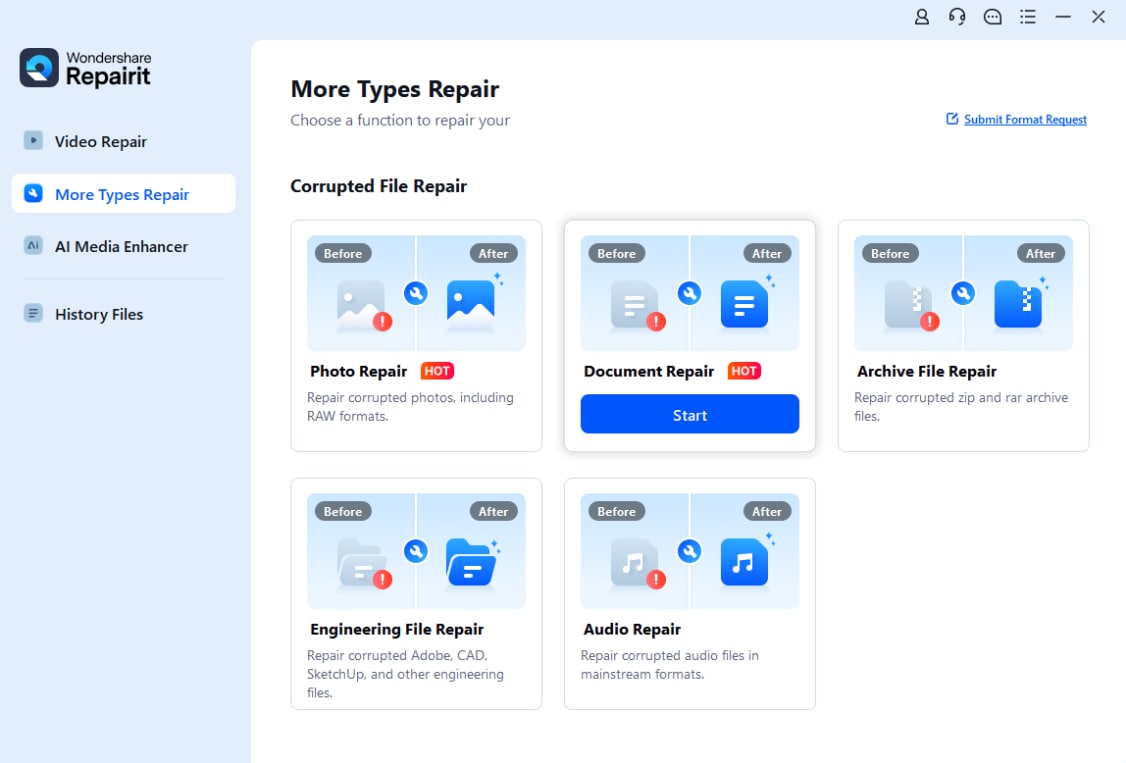
Step 1: Download and install Repairit on your computer. After setup the app, go to More Types Repair from the left side navigation pane, then select File Repair.

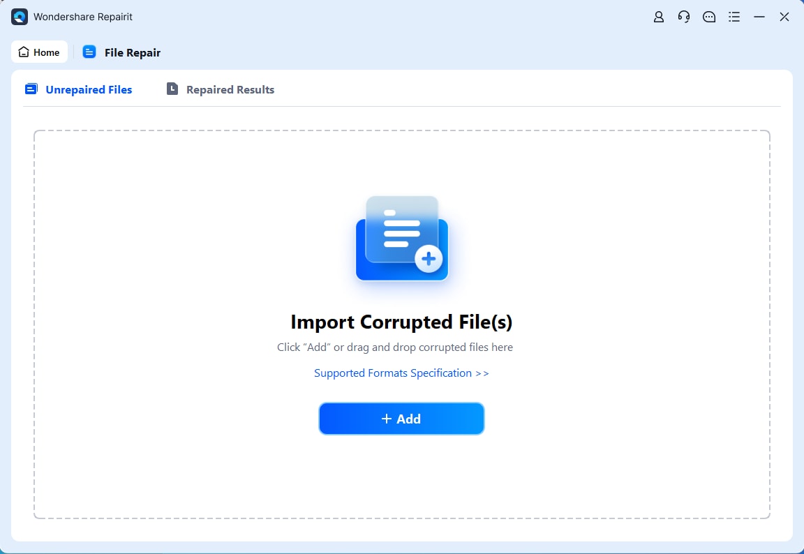
Step 2: Click + Add to choose an Excel file from your local storage. You can also upload multiple Excel files for batch repair.

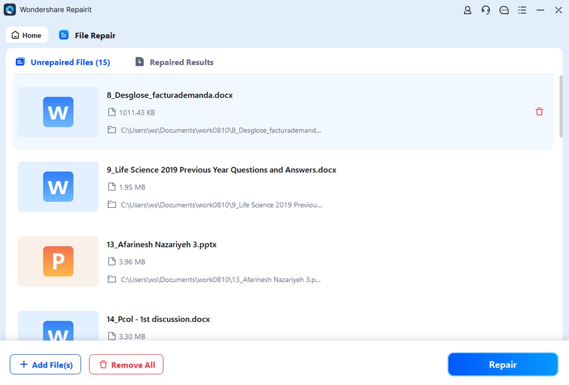
Step 3: Click Repair in the bottom-right corner of the screen to start the process.

Step 4: Preview results using the file icon Preview button before saving.

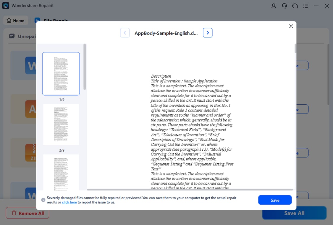
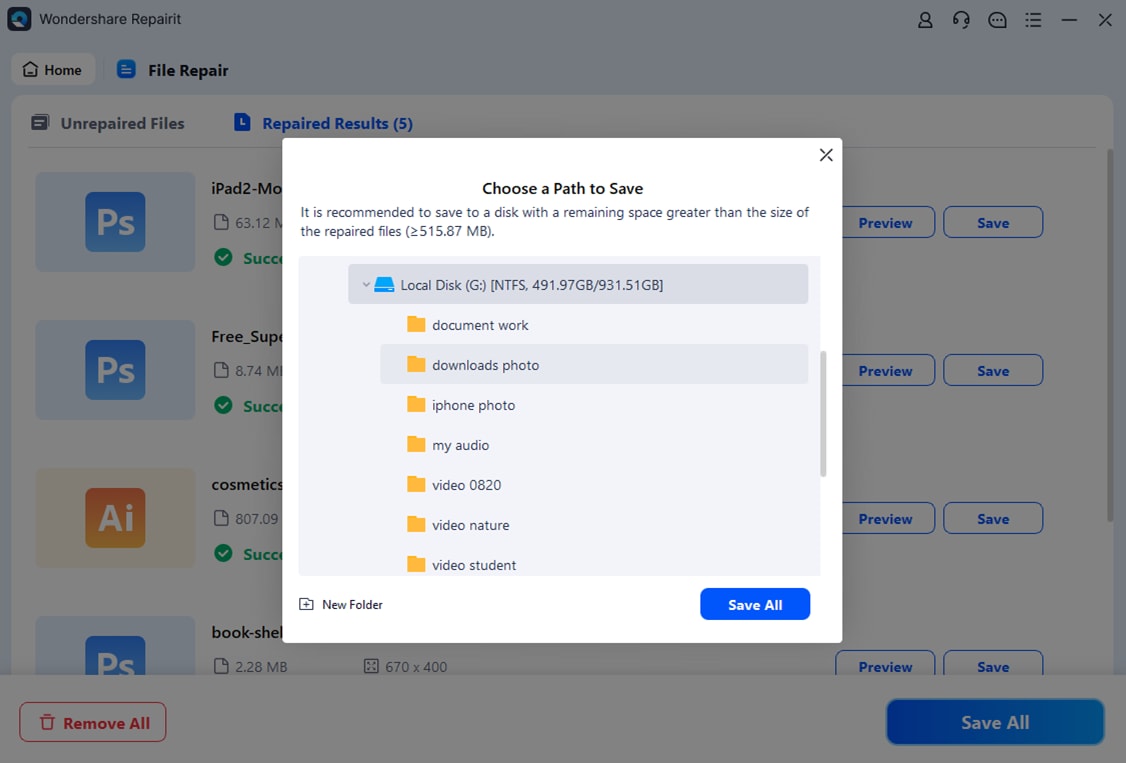
Step 5: Click Save or Save All to export the fixed Excel document. Choose your export location, and the app will save your files, showing progress on the screen.

This video can help you fix your excel files with a step-by-step guide.

Explore XLOOKUP

If you’re using Excel 365 or later, consider XLOOKUP. It’s more versatile, handles multiple tables, and even supports wildcards for partial matches.

Embrace Error Checking and Conditional Formatting

Use functions like IFERROR to highlight potential issues with conditional formatting. It makes your Excel spreadsheets easier to understand and troubleshoot.

Try On a Small Sample of Data

Test your VLOOKUP formulas on a small sample of data before applying them to your entire dataset. It helps identify errors and ensures the formula works as expected before you invest time and effort in broader applications.

Lock in Your Table Range With Absolute References

Use absolute references (e.g., $A$1) for the table range in your VLOOKUP formula. It ensures it stays anchored to the right spot even when copied or dragged.

Ensure Case Sensitivity With EXACT

Use the EXACT function within VLOOKUP to guarantee precise matches if your data is case-sensitive. It prevents unexpected results due to capitalization differences.

Enable Approximate Matches

Set the range_lookup argument in VLOOKUP to TRUE if you need to find approximate matches when the exact value isn’t present. However, be cautious, as this can lead to unintended results if not used carefully.

Conclusion

To wrap things up, you need to understand the issues with VLOOKUP when dealing with data. Knowing common problems helps you tackle any challenges that come your way.

By now, you have an idea of how to solve the most common problem in Excel VLOOKUP. Exploring these solutions ensures smoother data lookup experiences for you. Additionally, considering advanced solutions enhances efficiency in handling spreadsheet tasks. Wondershare Repairit stands out for resolving file-related concerns effectively. So, keep practicing your spreadsheet skills while confident that you can easily fix corrupted documents.