Everything You Need to Know About Excel Pivot Tables and Charts

In a world full of information, consider Excel Pivot Tables as your helpful friends. They excel at sorting out the data mess. These tools make it easy to organize, analyze, and understand information. By figuring out what they do and getting good at using them, you can move through your data without problems.

In this guide, we'll talk about Microsoft Excel's Pivot Tables and Charts - what they are and how to make them. Keep reading to find out more!

What Are Pivot Tables?

Before making Pivot tables, let us understand their uses, significance, and importance. Excel Pivot Tables are powerful data analysis tools. They enable us to easily summarize and analyze datasets. They allow you to rearrange and manipulate data. This provides a dynamic way to extract valuable insights. These are some benefits that Pivot Tables bring to data analysis:

1. Making Data Analysis Easier: Pivot Tables are like superheroes for easy data analysis. They help organize information. This makes it easy to spot trends and important details in your data.
2. Creating Interactive Reports: Pivot Tables are also awesome for creating reports that change with your data. You can get real-time insights, helping you make smart decisions quickly.
3. Efficient Summarization: Another cool thing about Pivot Tables is they can quickly summarize lots of data. Whether it's sales numbers, survey answers, or anything else, Pivot Tables make big sets of information easy to understand.
4. User-Friendly Data Exploration: With Pivot Tables, exploring and understanding data is like a fun adventure. You can drag and drop things around to see different angles of your information, helping you get what's going on underneath.

Pivot Tables Fundamentals

After understanding the significance and use of Excel Pivot Tables, let’s delve into the fundamental concepts. These concepts lay the groundwork for effective data analysis. They are the building blocks defining how your data is presented and analyzed. Here are the essential components of an Excel Pivot Table. They make it a versatile and powerful tool.

• Four Crucial Areas: Pivot tables revolve around four key areas – rows, columns, values, and filters. These components serve as the cornerstone, orchestrating the organization of your data. They also determine the metrics under scrutiny.
• Rows and Columns Categorize Data: Picture rows and columns as labels on arranged boxes. They categorize your data effortlessly. For instance, envision segregating sales by different products (rows) and regions (columns).
• Filters Refine Analysis: Filters act as magnifying glasses, allowing you to focus on specific criteria. Want to focus on sales data for a particular region? A filter provides that precision.
• Versatility in Data Sources: Pivot tables aren't confined to Excel sheets alone. They integrate with external databases and even online data. Think of it as a super-adaptable tool. It's ready to handle information from various sources.

Step-by-step of Creating Pivot Tables in Excel

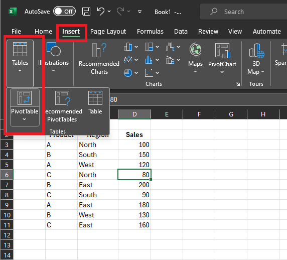
Step 1: Begin by selecting any cell within your dataset. This step signals Excel the area you want to analyze.

Step 2: Head to the "Insert" tab, then click on "Tables," and select "Pivot Table." This initiates the Pivot Table creation process.

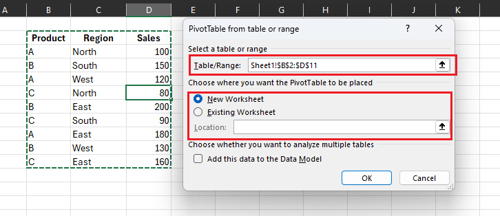
Step 3: Once you've selected "Pivot Table," a dialog box appears. The default settings usually work well, but here are a couple of things to consider:

1. Table/Range: Excel populates this based on your data set. Excel identifies the correct range if your data has no blank rows/columns. You can adjust this manually if necessary.
2. Choose the Location: Decide where you want the PivotTable report placed. If specific, specify the location. Otherwise, Excel creates a new worksheet with the Pivot Table.

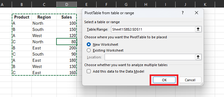
Step 4: Confirm your choices by clicking OK. Immediately, Excel generates a new worksheet, housing your created Pivot Table

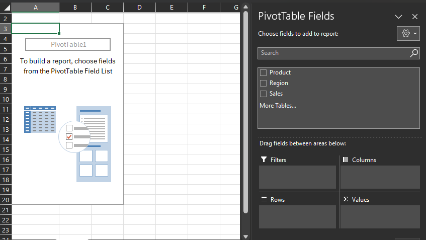
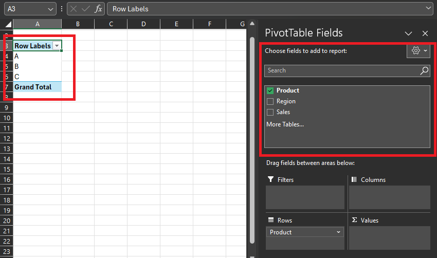
Once created, you'll notice the Pivot Table initially appears empty. The worksheet contains the Pivot Table name and a brief instruction line on the left. On the right, you'll find the Pivot Table Fields.

Tips for Those New to Pivot Tables in Excel

If this is your first time making pivot tables, I understand that the new information might be overwhelming and intimidating. But fret not. It is normal, and here are some tips for you.

1. Navigate the Pivot Table Field List with Confidence: Don't be intimidated by this list. It's your guide, and you can use it to pick and choose what you want to see in your pivot table.
2. Drag and Drop for Customization: This is where the fun begins. To customize your table, drag fields from the PivotTable Field List to areas like rows or columns. It's as easy as moving icons on your screen.
3. Common Challenges and Solutions: For beginners, selecting the correct data range poses a common challenge. Additionally, understanding the role of each field can be another hurdle. Think of it as ensuring you're working with the right information set. Also, understand what each piece of information does.

Creating and Using Pivot Charts in Excel

Pivot charts represent pivot table data, making trends and patterns more accessible. This visual element is especially useful for presenting data to stakeholders. It also facilitates making data-driven decisions.

Step-by-step guide in generating Pivot Charts

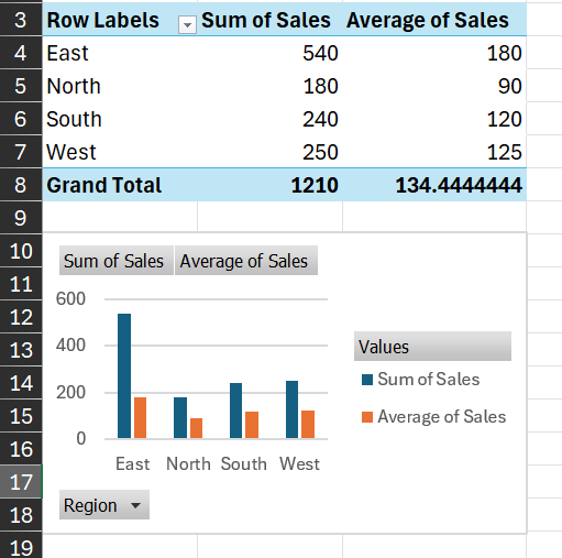
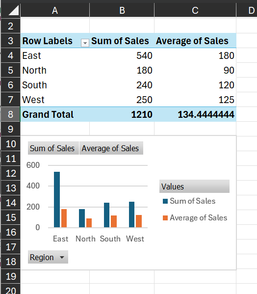
Step 1: Ensure you have a Pivot Table summarizing the data you want to visualize. In this case, we will be using the table for sales earlier.

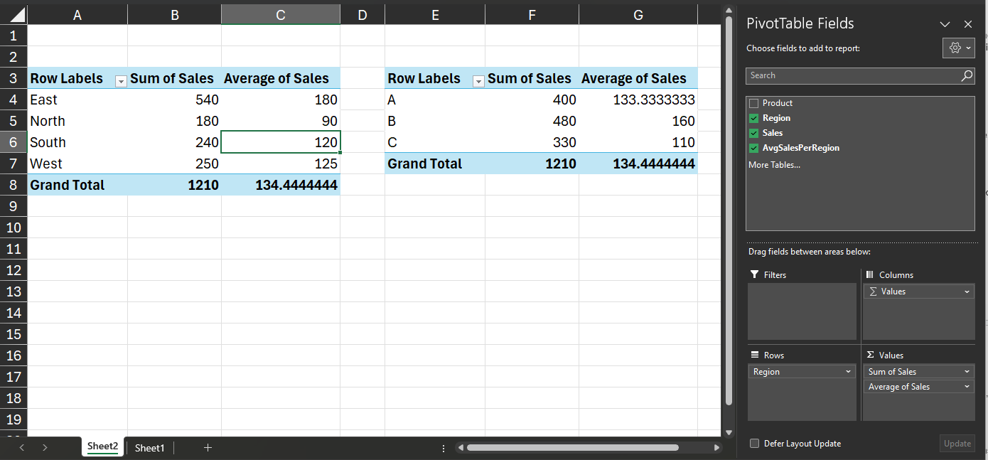
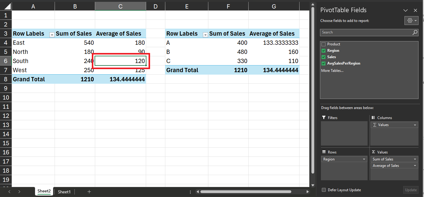
Step 2: Click on any cell within your existing Pivot Table. This step ensures that Excel recognizes the table you want to visualize.

Step 3: Head to the "Insert" tab in Excel, located in the top menu. You'll find various chart types within the "Charts" group, such as Bar Chart, Line Chart, or Pie Charts.

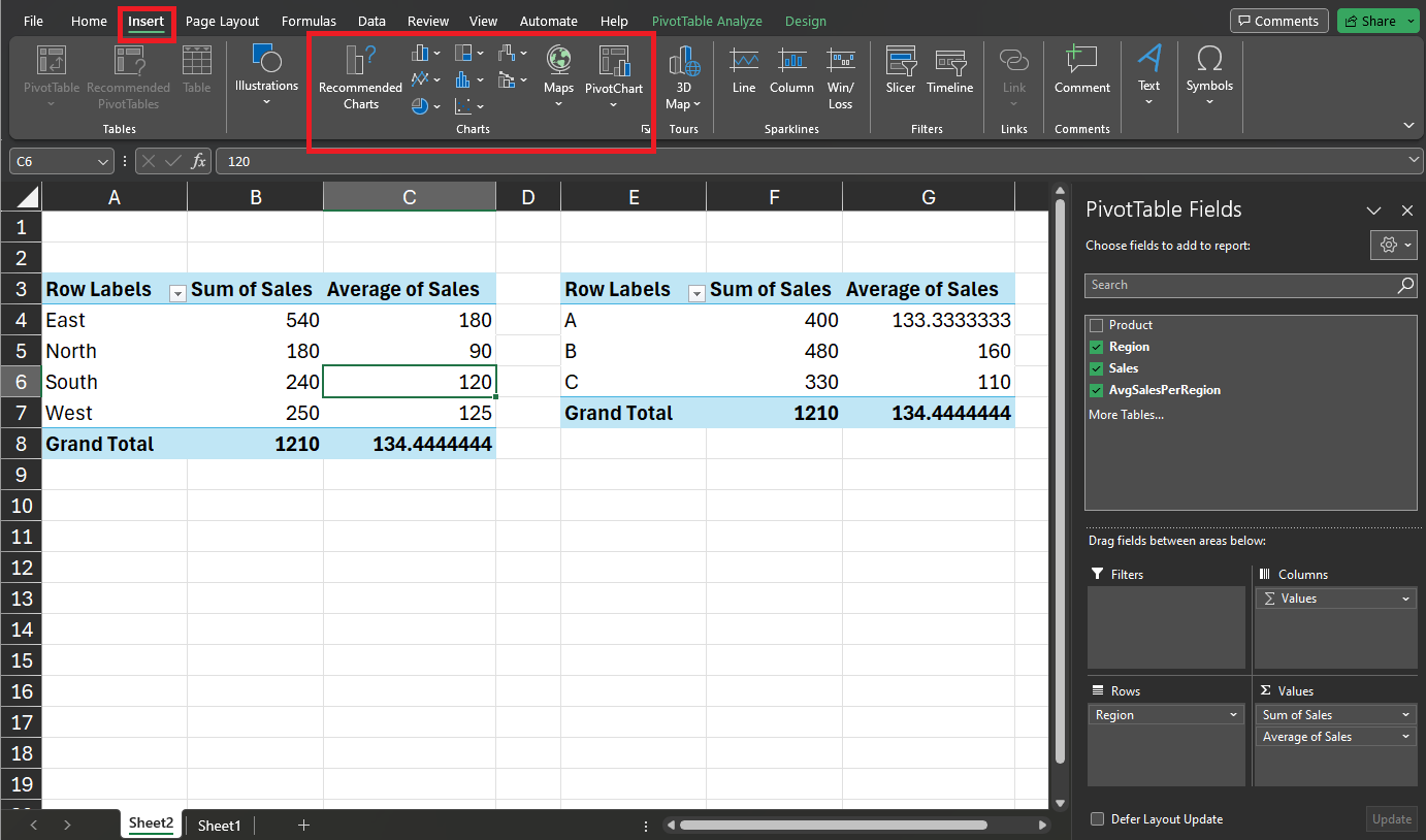
Step 4: Click on the desired chart type based on the nature of your data and the insights you want to convey.

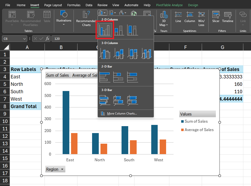
Excel will generate a chart Image nameed to your Pivot Table.

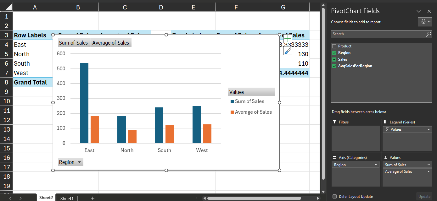
Step 5: Once you generate the chart, further customize it to enhance clarity. This customization also adds to its visual appeal. Adjust chart elements, titles, and labels to align with your analytical narrative.

Step 6: Excel provides various tools and options specific to charts. Explore features like data labels, legends, and trendlines to refine your visual representation. When selecting the chart, use the "Chart Tools" contextual tabs for more advanced customization.

Dynamic Updates: Image nameing Pivot Charts to Tables

One of the compelling features of Pivot Charts is their ability to maintain a dynamic Image name with underlying Pivot Tables. This Image name ensures that the chart reflects changes made in the associated tables in real time. Here's a step-by-step guide to Image name Pivot Charts to Tables.

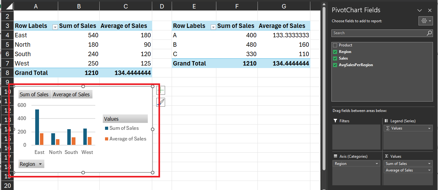
Step 1: Before establishing a Image name, ensure you have a Pivot Table and a corresponding Pivot Chart. Follow the steps outlined in the previous sections to create these elements.

Step 2: Click on any part of your existing Pivot Chart to select it. This action ensures Excel recognizes the specific chart you want to Image name to the Pivot Table.

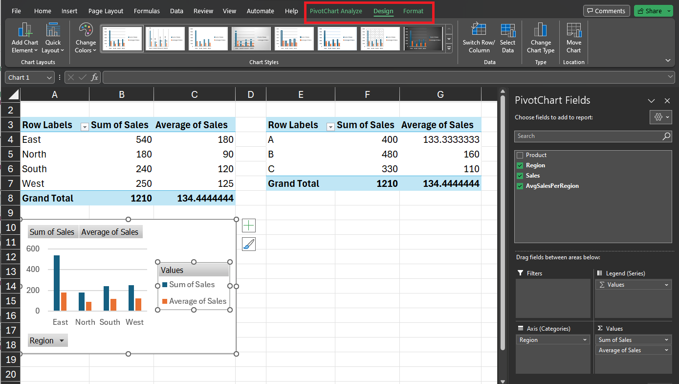
Step 3: Navigate to the "Analyze" tab (Excel 2013 and later) or the "Chart Tools" tab (Excel 2010) that appears when the chart is selected. Look for the option related to data or data source; it may vary depending on your Excel version.

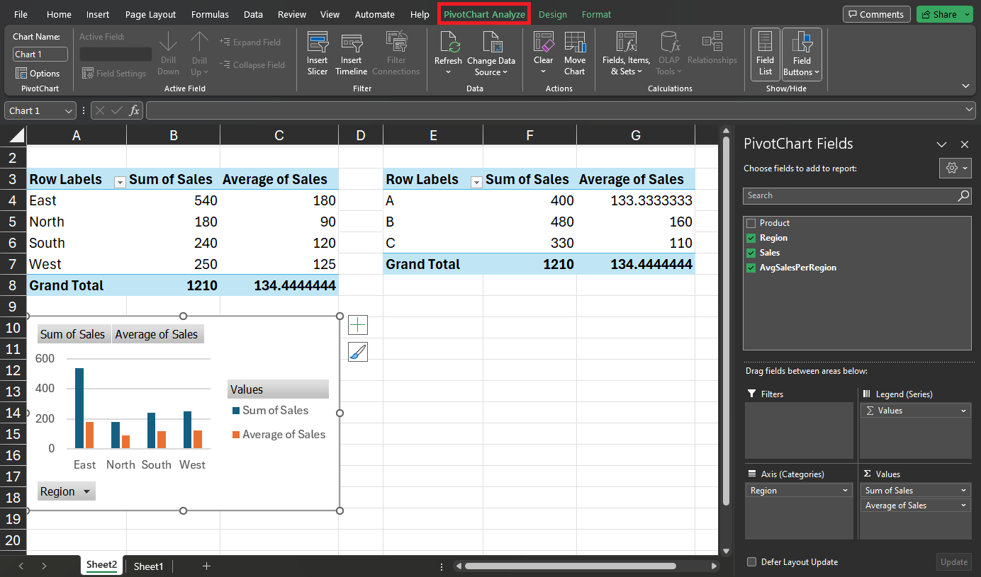
Step 4: In the "Analyze" or "Chart Tools" tab, find and select the "Select Data" option. This opens a dialog box.

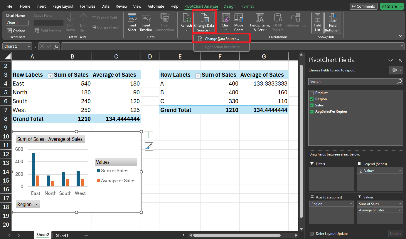
Step 5: Within the "Select Data Source" dialog box, you should see an option to add, edit, or remove a data source. Choose the "Add" or "Edit" option and select the range of your Pivot Table as the data source.

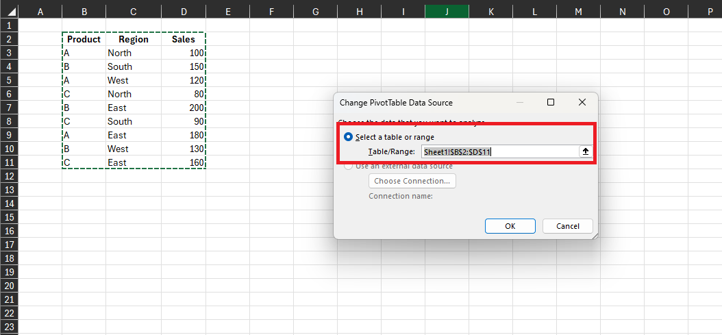
Step 6: Confirm your choices, and Excel will establish the Image name between the Pivot Chart and Table. As a result, any changes made to the underlying Pivot Table are now reflected in the Image nameed chart.

Repairing Damaged Pivot Table and Charts of Excel File

If you've encountered issues with your Excel Pivot Tables, Repairit File Repair Desktop is here to help. It's a reliable solution for identifying errors and resolving them. Additionally, it is effective for restoring damaged or corrupted files. Whether you're dealing with unexpected changes in file layout, inaccessible content, or files that won't open, Repairit can tackle these problems.

Wondershare Repairit handles corrupted files in Word, Excel, PowerPoint, and PDF formats. It ensures that the repair process doesn't alter the original content and supports various file formats. While Repairit is great for fixing files in different formats, it also does an excellent job repairing Pivot Tables and Charts within Excel files.

Wondershare Repairit - File Repair

Try It Free Try It Free

751,557 people have downloaded it.

• Repair damaged files with all levels of corruption, including blank files, files not opening, unrecognizable format, unreadable content, files layout changed, etc.

• Support to repair all formats of PDF, Word, Excel, PowerPoint, Zip, and Adobe files.

• Perfectly repair corrupted files with a very high success rate, without modifying the original file.

• No limit to the number and size of the repairable files.

• Support Windows 11/10/8/7/Vista, Windows Server 2003/2008/2012/2016/2019/2022, and macOS 10.10~macOS 13.

Features

• This tool effortlessly repairs corrupted files in different formats.
• Its user-friendly interface ensures a smooth experience, minimizing time and effort.
• With Repairit, you can preview repaired files before downloading them to ensure they meet your expectations.
• Take advantage of Repairit's batch-processing feature to simultaneously upload and repair many files.

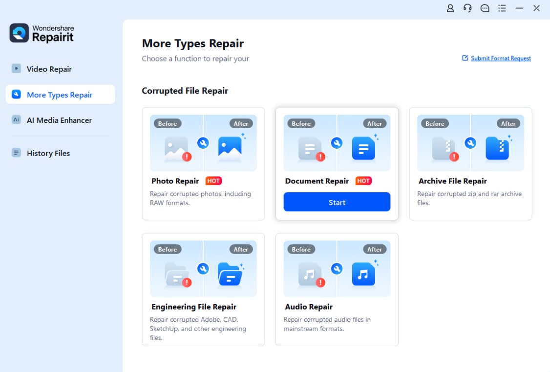
Step 1: Open Wondershare Repairit on your computer. Then, select "File Repair" under the "More Types Repair" section.

Add the damaged Excel files by clicking "Add."

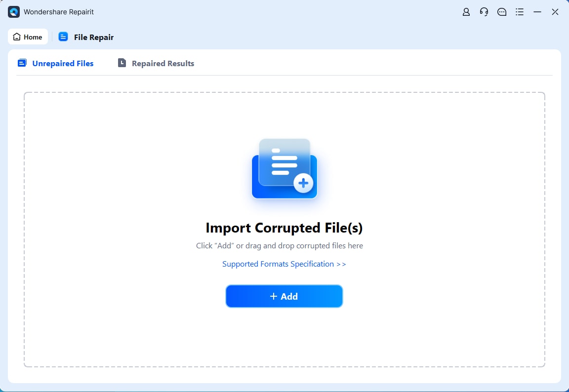
Tip: Repairit's batch-processing feature allows you to upload and repair many documents of various formats.

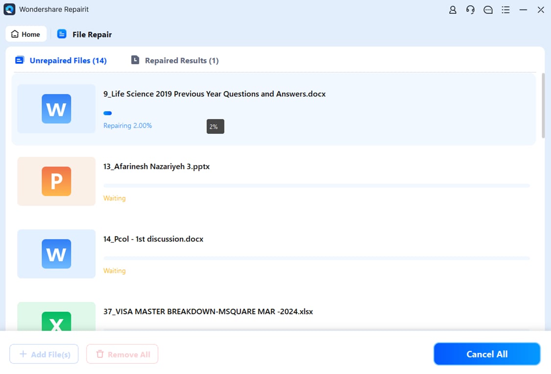
Step 2: After uploading the corrupted files, click "Repair" to start the repair process. Wait for the application to load and fix the files, then click "OK."

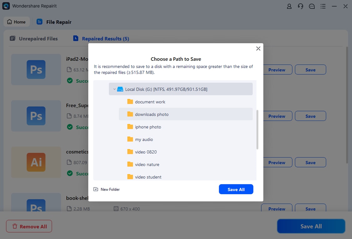
Step 3: A list of repaired files will appear. Preview the results by clicking the "Preview" button or the thumbnails. If satisfied with the results, click "Save" to save the repaired files. Or, go back, select multiple files, and use "Save All" to save them.

Note: For a more convenient and faster solution, especially if you only need to repair a few files with a size of 300 MB and below, consider using Repairit File Repair Online instead of the desktop version.

Conclusion

This guide has tackled the essentials of Excel Pivot Tables, covering basic creation. It has also explored advanced techniques such as leveraging functions and Power Pivot. Excel Pivot Tables offer powerful capabilities for informed decision-making and impactful data analysis. Whether you're a beginner or an advanced user, these tools are valuable for enhancing your skills. If you have ever encountered errors on your Pivot Tables and Charts, consider using Wondershare Repairit File Repair.